 Loop Catalog
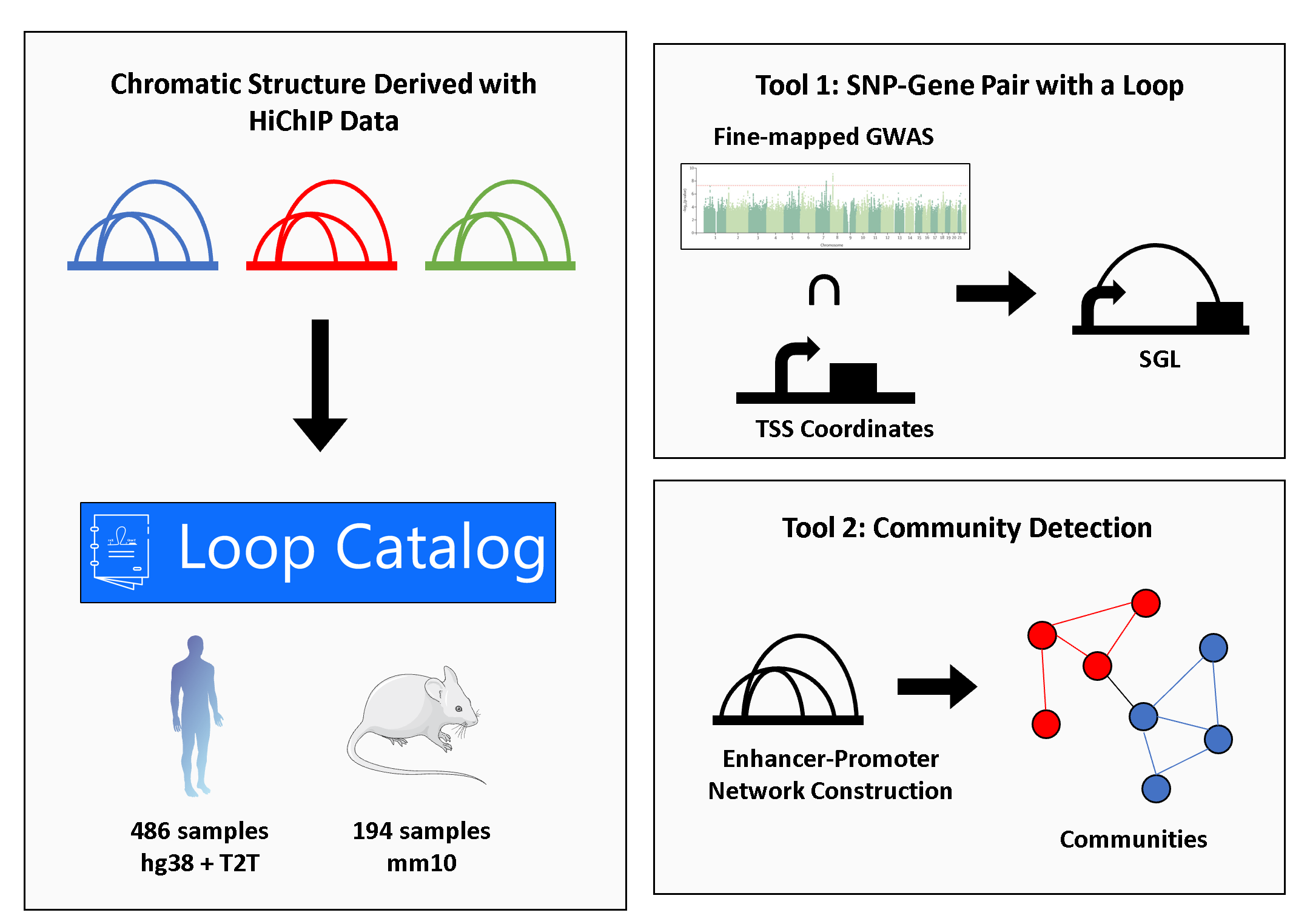
At the core of the Loop Catalog is HiChIP data from publically avaiable sources that are pulled together and processed uniformly (left). Our database is further expanded by additional analyses of which we make SGLs (Tool 1) and Community Detection (Tool 2) available.
To identify a comprehensive list of publicly-released HiChIP datasets, we scan NCBI’s Gene Expression Omnibus (GEO) database for studies performing HiChIP experiments. To extract information on these studies the Entrez and metapub.convert packages are used. Raw sequencing data associated to these studies is then identified from the SRA database using the pysradb Python package and the results are manually examined to extract HiChIP samples. ChIP-seq samples corresponding to these studies were also extracted if there is a record of them within the same GEO ID as the HiChIP sample.
To automatically add metadata, such as organ and cell type, to the curated HiChIP data, the BioPython.Entrez package was used to perform a search query within the GEO database. GSM IDs from the previous query were used with an esummary query to the biosample database. From these results organism, biomaterial, celltype, GSM ID, SRA ID, disease, organ, treatment, tissue, and strain (only for mouse) were extracted. “N/A” was used to indicate fields that are not applicable for a given sample and for the remaining fields, “Undetermined” was assigned when the information could not be retrieved. For cell lines, we provide additional detail by querying the Cellosaurus API.
HiChIP FASTQ files were systematically downloaded using one of three methods and prioritized in the following order: SRA-Toolkit’s prefetch and fasterq-dump (2.11.2), grabseqs (0.7.0), or EBI URLs generated from SRA Explorer (1.0). In addition, FASTQ files for phs001703v3p1 and phs001703v4p1 were downloaded that pertain to two previously published HiChIP studies from the Database of Genotypes and Phenotypes (dbGaP). Additionally, ChIP-seq FASTQ files were downloaded from GEO using grabseqs.
Our previously developed ChIPLine pipeline was used to align ChIP-seq reads with Bowtie2 and call calls peaks using MACS2 (2.2.7.1). If available, the corresponding input ChIP-seq files were used by MACS2 in ChIPLine for peak calling using input vs treatment mode. MACS2 peak calls were made without an input file if no such file was available for the sample. For ChIP-seq datasets with multiple biological replicates, the replicate with the larger number of peak calls was selected as the peak set to be used in downstream analyses for loop calling.
In the absence of matching ChIP-seq data, it is necessary to call peaks using HiChIP data. To achieve this, sets of peaks were inferred from HiChIP data using the FitHiChIP peak calling utility (10.0) that takes valid read pairs generated by HiCPro as input (i.e., one valid read pair corresponds to two individual reads). This tool also utilizes MACS2 for peak calling as mentioned above for ChIPLine. Peak calling was run using the PeakInferHiChIP.sh command by specifying the correct HiCPro output directory, reference genome, and read length as reported by SRA Run Selector entry for a given sample. If read lengths were different across technical replicates for a given HiChIP biological replicate, the mode read length was used. If no single mode read length existed, the greatest read length was selected. For merged biological replicates, the mode read length of all individual biological replicates for a given sample was chosen. Similarly, the highest read length was selected in the case that no single mode existed. Another tool, HiChIP-Peaks (0.1.2), was also used for peak calling but due its peak calls spanning untypically large-sized genomic regions (median 2.15 kb and up to 122 kb) with its default parameters, we decided to not utilize these peak calls.
Peaks called from ChIP-seq datasets were considered the ground truth set and peaks inferred directly from HiChIP datasets were assessed for their overlap with such ChIP-seq peaks. To measure the validity of HiChIP-inferred peaks, we calculated recall as the percentage of ChIP-seq peaks overlapped by at least one HiChIP-inferred peak. To obtain the intersection, each pair of corresponding HiChIP and ChIP-seq peak sets were intersected using bedtools allowing for 1kb slack on both sides.
Human samples were aligned to hg38 and t2t-chm13v2.0 while mouse samples were aligned to mm10 using the HiCPro (3.1.0) pipeline. Reference genomes were downloaded for hg38 (link), for mm10 (link) and for t2t-chm13 (link), and indexed with bowtie2 (2.4.5) using default parameters. All technical replicates were grouped into their respective biological replicate before read alignment. Restriction enzymes and ligation sequences were determined during the HiChIP literature search (Supp Table: REs) and restriction fragments were generated with the HiC-Pro digestion.py tool using default parameters. HiCPro was then run in parallel mode by splitting FASTQ files into chunks of 50,000,000 reads using HiCPro’s split_reads.py utility with a minimum MAPQ threshold of 30. HiC-Pro generated contact maps at the 1kb, 2kb, 5kb, 10 kb, 20kb, 40kb, 100kb, 500kb, and 1Mb resolutions. For all other HiCPro configuration parameters, the defaults were used.
All sets of HiChIP biological replicates for both human and mouse datasets originating from the same study and cell type were identified. Before merging the biological replicates, the reproducibility was assessed using hicreppy (0.1.0) which generates a stratum-adjusted correlation coefficient (SCC) as a measure of similarity for a pair of HiChIP contact maps. Briefly, contact maps in hic format were converted to cool format for hicreppy input at 1kb, 5kb, 10kb, 25kb, 50kb, 100kb, 250kb, 500kb, and 1mb resolutions using hic2cool (0.8.3). hicreppy was run on all pairwise combinations of replicates from a given HiChIP experiment. First, hicreppy htrain was used to determine the optimal smoothing parameter value, or h, for a pair of input HiChIP contact matrices at 5kb resolution. htrain was run on a subset of chromosomes and with a maximum possible h-value of 25. Default settings were used otherwise. Next, hicreppy scc was ran to generate a SCC for the matrix pair using the optimal h-value reported by htrain and at 5kb resolution considering chromosomes 1, 10, 17, and 19 only. A group of biological replicates were merged if all pairwise combinations of replicates in that group possessed a SCC greater than 0.8. Merging of biological replicates was performed by concatenating the corresponding HiCPro validpairs files before the peak and loop calling steps on these merged files.
Loop calling was performed for individual HiChIP biological replicates by (a) HiCCUPS (JuicerTools 1.22.01), (b) FitHiChIP with HiChIP-inferred peaks by FitHiChIP’s peak calling utility, and (c) FitHiChIP with ChIP-seq peaks, when available. Briefly, HiCPro validpairs files for each sample were converted to .hic format using HiCPro’s hicpro2juicebox utility with default parameters. HiCCUPS loop calling was initially performed for chr1 with the following parameters: --cpu, --ignore-sparsity, -c chr1, -r 5000,10000,25000, and -k VC. For samples that pass the chr1-specific thresholds of at least 200 loops for human samples and at least 100 loops for mouse samples (both at 10kb resolution) were then processed further with HiCCUPS for genome-wide loop calling using the same parameters. FitHiChIP loop calling was run with HiCPro validpairs as input at the 5kb, 10kb, and 25kb resolutions for the Stringent (S) background model with coverage bias regression, merge filtering, peak-to-all interactions and an FDR threshold of 0.01. Default values were used for all other FitHiChIP parameters.
SGLs were identified utilizing fine-mapped GWAS SNPs from CAUSALdb for Type 1 Diabetes (T1D), Rheumatoid Arthritis (RA), Psoriasis (PS), and Atopic Dermatitis (AD) which included 7, 7, 3, and 1 individual studies, respectively. The fine-mapped data was downloaded and lifted over from hg19 to hg38 using the MyVariantInfo Python package. As a proxy for promoters we downloaded the GENCODE v30 transcriptome reference, filtered transcripts for type equal to “gene” and located coordinates of the transcription start site (TSS). For genes on the plus strand, the TSS would be assigned as a 1bp region at the start site and, for the minus strand, the 1bp region at the end site. Lastly, we extracted all HiChIP samples whose cell type includes any of the following: T-cells, B cells, monocytes, and natural killer cells that resulted in 116 samples. To integrate these datasets, loop anchors were intersected with fine-mapped GWAS SNPs and promoters independently using bedtools pairtobed. Subsequently, loops were extracted as an SGL if at least one anchor contained a GWAS SNP and the opposing anchor contained a promoter.
To construct a network from chromatin loops, each anchor was considered a node and each significant loop an edge. In addition, anchors were labeled as promoters by intersecting with TSS coordinates (slack of +/- 2.5kb) and allowing the promoter label to take priority over any other possible label. For H3K27ac HiChIP data, non-promoter nodes/anchors are labeled as enhancers when they overlap with ChIP-seq peaks (no slack). All other nodes that are not a promoter or an enhancer were designated as “other”. After obtaining the annotated anchors, we created a weighted undirected graph using the loops as edges and loop strength as edge weights calculated as \the -log10(q-value) of FitHiChIP loop significance. To trim outliers, we set values larger than 20 to 20 and further scaled these values to between 0 and 1 for ease of visualization.
Community detection was applied to the networks created using FC loops at 5kb. Two levels of community detection were applied, the first detected communities within the overall network created for each chromosome (high-level) followed by a second round that detected subcommunities of the communities reported in the first round (low-level). High-level communities were located by running the Louvain algorithm using default parameters as implemented by the CDlib Python package. Starting with each high-level community, subcommunities were called using the same Louvain parameters. CRank was then applied at both levels to obtain a score that aggregates several properties related to the connectivity of a community into a single score for ranking.
The database is composed of two main parts, the first contains high sample-level and low-level loop information while the second contains SGL specific tables with auxiliary tables used to add additional annotations. For the first part we atomized the data into the following tables: hic_sample, celltype, hicpro, chipseq_merged, fithichip_cp, fithichip_cp_loop, hiccup, fithichip_hp and reference which allowed us to capture important metadata and the uniqueness of loops using different loop callers. The second part includes the gwas_study, gwas_snp, snp, gene and fithichip_cp_fm_sgls tables which allowed us to capture important relationships for SGLs and to facilitate their query. The full database schema can be found in Supplementary Figure XX.
Loop Catalog was built using Django v3.2 as the backend framework with all data stored using the Postgresql v9 database management system. To style the frontend interface, we used Bootstrap 5.2. For implementing advanced tables and charts DataTables v1.12.1, Charts.js v4.0, and D3 v4.13.0 were used. To visualize genetic and epigenetic data the WashU Epigenome Browser v53.6.3 was used which maintains an easily accessible web embedding. Lastly, CytoscapeJS v3.26.0 was used to visualize enhancer-promoter networks.